 |
 |
|
W-ChIPeaksA comprehensive web application for processing ChIP-chip and ChIP-seq data |
|


 |
 |
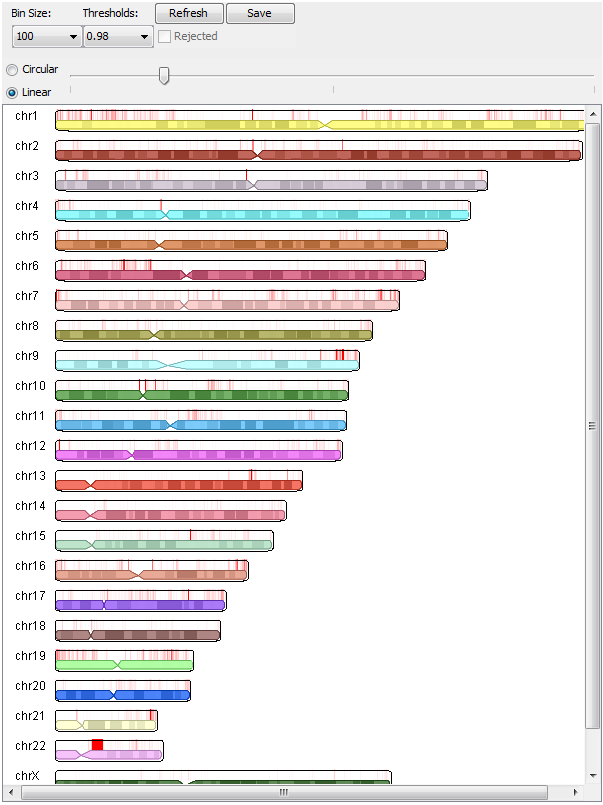
Graphical Display
How to useTo load the graphical display, click "Load Graphical Display" on the results page. If threshold percentages were specified, the results for each bin size and threshold specified can be selected via the "Bin Size:" and "Thresholds:" drop-down menus. If a target FDR was specified, choosing bin sizes will select the results file with peaks called with that bin size. If a control file was supplied, the "Rejected" checkbox will select the called peaks that were rejected based on the control file. Two scaling modes are available: circular and linear (described in detail below). The slider controls the intensity of the scaling to be performed. For circular scaling, the midpoint of the slider represents no scaling. Moving the slider to the left scales down called peaks, and moving it to the right scales up called peaks. For linear scaling, the left end of the slider represents no scaling, and moving the slider to the right scales up called peaks. After specifying the options for the graphical display, click on "Refresh". Images can be saved to disk by clicking on "Save", provided that the applet's digital certificate was accepted. The applet will still function even if the certificate is not accepted, although saving the image will not work. |
 |
Scaling details
The intensity of all peaks called by BELT is normalized to a [0, 1] scale by the BELT graphical display, and the chromosome images are generated directly from the scores without a scaling function. Two scaling functions are available: circular and linear. Circular scaling artificially increases or decreases midrange scores most strongly, and linear scaling artificially increases lower scores most strongly. Circular scaling tends to be most useful in distinguishing clusters of peaks with high intensity, and linear scaling tends to be most useful in viewing lower-intensity peaks in cases where a few peaks of very high intensity would otherwise dominate the [0, 1] intensity normalization.
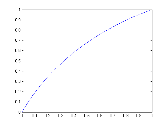
Both scaling functions map normalized raw peak scores to scaled peak scores, also on a [0, 1] scale, given a scale factor (set by the display's slider). For circular scaling, the scale factor is the radius of a circle, and the scaling function is the segment of the circle at a 45° angle in quadrant II if positive and quadrant IV if negative. For linear scaling, the function is a straight line passing through (1, 1) with slope [0, 1] defined by the scale factor.
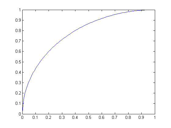
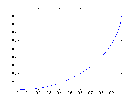
For all graphs below, the raw score is the independent variable and the scaled score is the dependent variable.
 |
 |
| Circular scaling function for radius 1 (a quarter-circle) | Circular scaling function for radius -1 |
 |
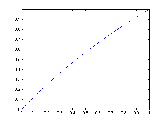 |
| Circular scaling function for radius 2 | Circular scaling function for radius 3 |
 |
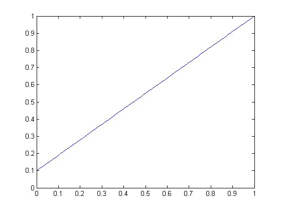 |
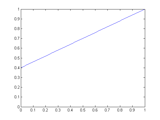
| Linear scaling function for slope 0.6 | Linear scaling function for slope 0.9 |
For circular scaling (all angles in radians):
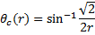 , where θc is equal to one-half the angle of the circle used.
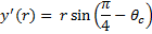 , where y' is equal to the y offset necessary so that the portion of the circle used is within ([0:1], [0:1]).
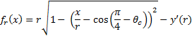 , where fr(x) is the circular scaling function for raw score x and radius r.
For linear scaling:
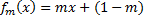 , where fm(x) is the linear scaling function for raw score x and slope m.